Peptide workflow with DaparToolshed
Manon Gaudin
Samuel Wieczorek
Thomas Burger
2026-02-05
Source:vignettes/DaparToolshed.Rmd
DaparToolshed.RmdIntroduction
DaparToolshed is a package for analyzing quantitative
data from label-free bottom-up proteomics experiments. It uses
MultiAssayExperiment, SummarizedExperiment and
QFeatures data structures (Gatto and
Vanderaa (2025)).
Starting from a table of abundance values and associated metdata,
DaparToolshed proposes functions to build a complete
statistical analysis workflow up to the selection of differentially
expressed proteins in the contrasted conditions.
DaparToolshed makes it possible to import data at different
levels: precursor, peptide or protein, each requiring specific
processing.
This vignette describes a complete precursor- or peptide-level workflow.
This package is used by the Prostar2 package, which
provides a user-friendly graphical interfaces, so that programming skill
is not required to achieve the data analysis.
Import dataset
For testing purposes, the DaparToolshedData package is
accompanied with several example datasets.
The dataset used in this vignette is an extract from the
Exp1_R25_pept dataset in the DaparToolshedData
package (Giai Gianetto et al. (2016)). It
comprises 500 peptides and 6 samples, divided into 2 conditions
(“25fmol” and “10fmol”).
data.file <- system.file("extdata/data", "Exp1_R25_pept_500.txt", package="DaparToolshed")
data <- read.table(data.file, header=TRUE, sep="\t", as.is=TRUE, stringsAsFactors = FALSE)

sample.file <- system.file("extdata/data", "samples_Exp1_R25.txt", package="DaparToolshed")
sample <- read.table(sample.file, header=TRUE, sep="\t", as.is=TRUE, stringsAsFactors = FALSE)
DaparToolshed uses MultiAssayExperiment,
SummarizedExperiment and QFeatures data
structures.
The function createQFeatures() allows for the
importation of a given dataset to a QFeatures format. The
dataset can come from any tabulated-like file containing quantitative
data and metadata, accompanied by another dataframe for the sample
description. The QFeatures format allows you to keep track
of the various transformations made at each step.
For each peptide (or precursor) in each sample of the dataset, it is
possible to tag the evidence that links the abundance to the molecule
identified: for instance, if the abundance value is missing or imputed,
if the quantification-identification match result from a transfer
between samples or if there has been a fragmentation spectrum identified
in relation to the quantified elution profile, etc. If such metadata is
available, then the corresponding column indexes can be indicated in
indexForMetacell. This allows the information to be
leveraged during the workflow. The quantitative data do not need to be
logged beforehand, as setting logData = TRUE will yield
automatic log-transform. Similarly, with force.na = TRUE,
any quantitative data with a null value or a NaN will be converted to
NA. It is necessary to specify the column of the table where the mother
proteins are indicated ('parentProtId' parameter) as an
adjacency matrix is created when the function is executed. This matrix
provides easy access to peptide-protein relationships, including shared
peptides, i.e., when the same peptide belongs to several proteins. To
run a peptidomics analysis (i.e., peptides are analysed irrespective of
their mother proteins), as no peptide-to-protein aggregation is
necessary, it is more suited to rely on the same workflow as for
protein-level analysis.
obj <- createQFeatures(data = data,
                       sample = sample,
                       indQData = 56:61,
                       keyId = "Sequence",
                       indexForMetacell = 43:48,
                       logData = TRUE,
                       force.na = TRUE,
                       typeDataset = "peptide",
                       parentProtId = "Protein_group_IDs",
                       analysis = "Pept_Data",
                       software = "maxquant",
                       name = "original")

obj
## An instance of class QFeatures (type: bulk) with 2 sets:
##
## [1] original: SummarizedExperiment with 500 rows and 6 columns
## [2] logAssay: SummarizedExperiment with 500 rows and 6 columnsThe data obtained includes two assays: original and
logAssay. The original, non-logged data is contained in
original, while the logged data is in
logAssay. This shows how the QFeatures format
allows for recording the state of the dataset after each step.
Filtering
The first step in this workflow is peptide filtering. Not all
peptides in the dataset are relevant for analysis. Some may be
contaminants, for example, while others may have too many missing values
to be taken into account. This filtering can be done using information
contained in quantitative data tags (see above) or metadata, i.e., all
the variables from the original dataset that were not quantitative data
and can be accessed through the
SummarizedExperiment::rowData() function.
##                           metacell_Intensity_C_R1 metacell_Intensity_C_R2
## AAAAQDEITGDGTTTVVCIVGEIIR     Quant. by direct id     Quant. by direct id
## AAADAISDIEIK                  Quant. by direct id     Quant. by direct id
## AAADAISDIEIKDSK                Quant. by recovery     Quant. by direct id
## AAAEEQAKR                             Missing POV     Quant. by direct id
## AAAEGVANIHIDEATGEMVSK         Quant. by direct id     Quant. by direct id
## AAAEYEKGEYETAISTINDAVEQGR     Quant. by direct id     Quant. by direct id
##                           metacell_Intensity_C_R3 metacell_Intensity_D_R1
## AAAAQDEITGDGTTTVVCIVGEIIR             Missing POV     Quant. by direct id
## AAADAISDIEIK                  Quant. by direct id     Quant. by direct id
## AAADAISDIEIKDSK               Quant. by direct id     Quant. by direct id
## AAAEEQAKR                             Missing POV             Missing MEC
## AAAEGVANIHIDEATGEMVSK          Quant. by recovery     Quant. by direct id
## AAAEYEKGEYETAISTINDAVEQGR     Quant. by direct id     Quant. by direct id
##                           metacell_Intensity_D_R2 metacell_Intensity_D_R3
## AAAAQDEITGDGTTTVVCIVGEIIR     Quant. by direct id     Quant. by direct id
## AAADAISDIEIK                  Quant. by direct id     Quant. by direct id
## AAADAISDIEIKDSK               Quant. by direct id     Quant. by direct id
## AAAEEQAKR                             Missing MEC             Missing MEC
## AAAEGVANIHIDEATGEMVSK         Quant. by direct id     Quant. by direct id
## AAAEYEKGEYETAISTINDAVEQGR Quant. by direct id Quant. by direct id## DataFrame with 3 rows and 61 columns
## Sequence N_term_cleavage_window
## <character> <character>
## AAAAQDEITGDGTTTVVCIVGEIIR AAAAQDEITG... PTAVIIARAA...
## AAADAISDIEIK AAADAISDIE... MPKETPSKAA...
## AAADAISDIEIKDSK AAADAISDIE... MPKETPSKAA...
## C_term_cleavage_window Amino_acid_before
## <character> <character>
## AAAAQDEITGDGTTTVVCIVGEIIR CIVGEIIRQA... R
## AAADAISDIEIK AISDIEIKDS... K
## AAADAISDIEIKDSK DIEIKDSKSN... K
## First_amino_acid Second_amino_acid
## <character> <character>
## AAAAQDEITGDGTTTVVCIVGEIIR A A
## AAADAISDIEIK A A
## AAADAISDIEIKDSK A A
## Second_last_amino_acid Last_amino_acid
## <character> <character>
## AAAAQDEITGDGTTTVVCIVGEIIR I R
## AAADAISDIEIK I K
## AAADAISDIEIKDSK S K
## Amino_acid_after A_Count R_Count N_Count
## <character> <integer> <integer> <integer>
## AAAAQDEITGDGTTTVVCIVGEIIR Q 4 1 0
## AAADAISDIEIK D 4 0 0
## AAADAISDIEIKDSK S 4 0 0
## D_Count C_Count Q_Count E_Count G_Count
## <integer> <integer> <integer> <integer> <integer>
## AAAAQDEITGDGTTTVVCIVGEIIR 2 1 1 2 3
## AAADAISDIEIK 2 0 0 1 0
## AAADAISDIEIKDSK 3 0 0 1 0
## H_Count I_Count L_Count K_Count M_Count
## <integer> <integer> <integer> <integer> <integer>
## AAAAQDEITGDGTTTVVCIVGEIIR 0 4 0 0 0
## AAADAISDIEIK 0 3 0 1 0
## AAADAISDIEIKDSK 0 3 0 2 0
## F_Count P_Count S_Count T_Count W_Count
## <integer> <integer> <integer> <integer> <integer>
## AAAAQDEITGDGTTTVVCIVGEIIR 0 0 0 4 0
## AAADAISDIEIK 0 0 1 0 0
## AAADAISDIEIKDSK 0 0 2 0 0
## Y_Count V_Count U_Count Length
## <integer> <integer> <integer> <integer>
## AAAAQDEITGDGTTTVVCIVGEIIR 0 3 0 25
## AAADAISDIEIK 0 0 0 12
## AAADAISDIEIKDSK 0 0 0 15
## Missed_cleavages Mass Proteins
## <integer> <numeric> <character>
## AAAAQDEITGDGTTTVVCIVGEIIR 0 2559.28 P39079
## AAADAISDIEIK 0 1215.63 P09938
## AAADAISDIEIKDSK 1 1545.79 P09938
## Leading_razor_protein Start_position End_position
## <character> <integer> <integer>
## AAAAQDEITGDGTTTVVCIVGEIIR sp|P39079|... 79 103
## AAADAISDIEIK sp|P09938|... 9 20
## AAADAISDIEIKDSK sp|P09938|... 9 23
## Unique_Groups Unique_Proteins Charges PEP
## <character> <character> <character> <numeric>
## AAAAQDEITGDGTTTVVCIVGEIIR yes yes 2;3 2.4684e-25
## AAADAISDIEIK yes yes 2 1.8883e-04
## AAADAISDIEIKDSK yes yes 3 2.7740e-06
## Score Experiment_C_R1 Experiment_C_R2
## <numeric> <integer> <integer>
## AAAAQDEITGDGTTTVVCIVGEIIR 114.150 1 2
## AAADAISDIEIK 63.662 1 1
## AAADAISDIEIKDSK 93.237 1 1
## Experiment_C_R3 Experiment_D_R1 Experiment_D_R2
## <integer> <integer> <integer>
## AAAAQDEITGDGTTTVVCIVGEIIR NA 2 2
## AAADAISDIEIK 1 1 1
## AAADAISDIEIKDSK 1 1 1
## Experiment_D_R3 Intensity Reverse
## <integer> <numeric> <logical>
## AAAAQDEITGDGTTTVVCIVGEIIR 2 153490000 NA
## AAADAISDIEIK 1 133190000 NA
## AAADAISDIEIKDSK 1 136500000 NA
## Potential_contaminant id Protein_group_IDs
## <character> <integer> <character>
## AAAAQDEITGDGTTTVVCIVGEIIR 0 1210
## AAADAISDIEIK 1 254
## AAADAISDIEIKDSK 2 254
## Mod_peptide_IDs Evidence_IDs MS_MS_IDs
## <character> <character> <character>
## AAAAQDEITGDGTTTVVCIVGEIIR 0 0;1;2;3;4;... 0;1;2;3;4;...
## AAADAISDIEIK 1 9;10;11;12... 8;9;10;11;...
## AAADAISDIEIKDSK 2 15;16;17;1... 14;15;16;1...
## Best_MS_MS Oxidation_M_site_IDs MS_MS_Count
## <integer> <character> <integer>
## AAAAQDEITGDGTTTVVCIVGEIIR 6 8
## AAADAISDIEIK 8 4
## AAADAISDIEIKDSK 14 5
## qMetacell
## <data.frame>
## AAAAQDEITGDGTTTVVCIVGEIIR Quant. by ...:Quant. by ...:Missing PO...:...
## AAADAISDIEIK Quant. by ...:Quant. by ...:Quant. by ...:...
## AAADAISDIEIKDSK Quant. by ...:Quant. by ...:Quant. by ...:...
## adjacencyMatrix
## <dgCMatrix>
## AAAAQDEITGDGTTTVVCIVGEIIR 1:0:0:...
## AAADAISDIEIK 0:1:0:...
## AAADAISDIEIKDSK 0:1:0:...To apply a filter based on tags, the FunctionFilter()
function should be used. The functions
QFeatures::filterFeature() and
QFeatures::VariableFilter() can be used to create filters
from metadata.
 #create filter to remove empty lines
filter_emptyline <- FunctionFilter("qMetacellWholeLine",
                                  cmd = 'delete',
                                  pattern = 'Missing MEC')

 #create filter to remove contaminant
filter_contaminant <- QFeatures::VariableFilter(field = "Potential_contaminant",
                                                value = "+",
                                                condition = "==",
                                                not = TRUE)
Doing so creates the filter but does not apply them to the data. All
created filters can be applied at once using the
filterFeaturesOneSE() function, which will perform
filtering on the assay indicated by i and create a new
assay with the filtered peptides.
 #apply all filters and create new assay
obj <- filterFeaturesOneSE(object = obj,
                           i = length(obj),
                           name = "Filtered",
                           filters = list(filter_emptyline, filter_contaminant))
It is advised to remove proteins that no longer have an associated peptide following this filtering from the adjacency matrix in order to facilitate the subsequent aggregation step.
 #remove proteins with no associated peptides
X <- SummarizedExperiment::rowData(obj[[length(obj)]])$adjacencyMatrix
SummarizedExperiment::rowData(obj[[length(obj)]])$adjacencyMatrix <- X[, -which(Matrix::colSums(X) == 0)]

obj
## An instance of class QFeatures (type: bulk) with 3 sets:
##
## [1] original: SummarizedExperiment with 500 rows and 6 columns
## [2] logAssay: SummarizedExperiment with 500 rows and 6 columns
## [3] Filtered: SummarizedExperiment with 480 rows and 6 columnsNormalization
The normalization step reduces biases introduced at any preliminary stage, as to make samples more comparable. Though not a full batch effect correction method (which can be required depending on the experimental design), it can limit some simple batch effects. During this step, peptide abundances are essentially rescaled between samples of the same conditions or of all conditions.
Several algorithms are implemented in DaparToolshed and
the list of available methods can be accessed by using
normalizeMethods() :
 #list of available methods
normalizeMethods()
## [1] "GlobalQuantileAlignment" "SumByColumns"
## [3] "QuantileCentering" "MeanCentering"
## [5] "LOESS" "vsn"The methods proposed acts as described below:
-
GlobalQuantileAlignment: Aligns the quantiles of intensity distributions across all samples. (This method should be used cautiously, as it imposes a high-impact normalization. Broadly speaking, the abundances are replaced by their order statistics). -
SumByColumns: Normalizes each abundance value by the total abundance of its corresponding sample. Un-logged intensities are used for processing. This method assumes the total amount of biological material is equal in all the samples . -
QuantileCentering: Aligns the intensity distributions to a specific quantile, e.g., the median or a lower quantile, either across all samples or within each condition. -
MeanCentering: Aligns the intensity distributions to their means, either across all samples or within each condition. Optionally, unit variance can be enforced. -
LOESS: Applies a cyclic LOESS normalization, either across all samples or within each condition. The intensity values are normalized by means of a local regression model of the difference of intensities as function of the median intensity value (Cleveland (1979)) (see Smyth (2005) for implementation details). -
vsn: Applies the Variance Stabilization Normalization method, either across all samples or within each condition (Huber et al. (2002)).
The normalizeFunction() function allows you to normalize
data using any of the methods described above and create a new assay
with normalized data. The parameters to be defined depend on the chosen
method. The type argument allows to indicate whether the
method is applied to the entire dataset at once ("overall")
or whether each condition is normalized independently
("within conditions").
obj <- normalizeFunction(obj,
                         method = "MeanCentering",
                         scaling = TRUE,
                         type = "overall")

obj
## An instance of class QFeatures (type: bulk) with 4 sets:
##
## [1] original: SummarizedExperiment with 500 rows and 6 columns
## [2] logAssay: SummarizedExperiment with 500 rows and 6 columns
## [3] Filtered: SummarizedExperiment with 480 rows and 6 columns
## [4] Normalization: SummarizedExperiment with 480 rows and 6 columnsThe compareNormalizationD_HC() function provides a way
to visually compare the quantitative data before and after
normalization. This plot shows the influence of the normalization
method.
obj1 <- obj[[length(obj)]]
obj2 <- obj[[length(obj)-1]]
protId <- DaparToolshed::idcol(obj1)

.n <- floor(0.02 * nrow(obj1))
.subset <- seq(nrow(obj1))

compareNormalizationD_HC(
  qDataBefore = SummarizedExperiment::assay(obj1),
  qDataAfter = SummarizedExperiment::assay(obj2),
  keyId = SummarizedExperiment::rowData(obj1)[, protId],
  conds = DaparToolshed::design.qf(obj)$Condition,
  n = .n,
  subset.view = .subset
)
Imputation
It is common to face a significant number of missing values. To overcome this problem, it is often necessary to resort to imputation. However, it is important to note that data imputation amount to creating experimental measurements out of thin air (and of a bit of mathematics too). It is thus recommended to avoid imputation whenever possible. However, most algorithms required subsequently cannot deal with missing values, and the few that claim to be robust to missing values either relies on implicit or explicit imputation, which makes them no better.
First, it is interesting to look at the quantity and distribution of
missing values. The metacellPerLinesHisto_HC() and
metacellPerLinesHistoPerCondition_HC() functions give
access to the number of rows containing a given number of missing
values, respectively for all samples and within each condition. These
functions use the quantitative data tags described above.
pal <- unique(GetColorsForConditions(design.qf(obj)$Condition))
pattern <- c("Missing MEC", "Missing POV")
grp <- design.qf(obj)$Condition

 #number of line with different amount of NA
metacellPerLinesHisto_HC(obj[[length(obj)]], group = grp, pattern = pattern)
 #number of line with different amount of NA per condition
metacellPerLinesHistoPerCondition_HC(obj[[length(obj)]], group = grp, pattern = pattern)
The hc_mvTypePlot2() function displays density plots
showing the distribution of partially observed values for each
condition. The x-axis corresponds to the mean intensity of a peptide in
a condition, while the y-axis indicates the number of observed values
for that peptide under the same condition.
It can be observed that the distribution tends to shift towards higher values when fewer missing values are present. This is a sign that at least some of the missing values originate from peptides that are below the lower limit of the mass spectrometer.
hc_mvTypePlot2(obj[[length(obj)]], group = grp, pattern = pattern, pal = pal)Numerous imputation methods exist. Here, data imputation is performed
using the wrapper.pirat() function, which is a wrapper for
the Pirat method. Pirat is an imputation
method that uses a penalized maximum likelihood strategy and accounts
for sibling peptide correlations (Etourneau et
al. (2024)). It does not require any parameter tuning. For more
information on this method, see the Pirat
package.
obj <- wrapper.pirat(data = obj,
                     adjmat = SummarizedExperiment::rowData(obj[[length(obj)]])$adjacencyMatrix,
                     extension = "base")
##
## Call:
## stats::lm(formula = log(probs) ~ m_ab_sorted[seq(length(probs))])
##
## Residuals:
## Min 1Q Median 3Q Max
## -1.7621 -0.4354 0.1148 0.4852 1.8991
##
## Coefficients:
## Estimate Std. Error t value Pr(>|t|)
## (Intercept) 24.07420 1.35105 17.82 <2e-16 ***
## m_ab_sorted[seq(length(probs))] -1.07882 0.05536 -19.49 <2e-16 ***
## ---
## Signif. codes: 0 '***' 0.001 '**' 0.01 '*' 0.05 '.' 0.1 ' ' 1
##
## Residual standard error: 0.6937 on 368 degrees of freedom
## Multiple R-squared: 0.5079, Adjusted R-squared: 0.5066
## F-statistic: 379.8 on 1 and 368 DF, p-value: < 2.2e-16
obj## An instance of class QFeatures (type: bulk) with 5 sets:
##
## [1] original: SummarizedExperiment with 500 rows and 6 columns
## [2] logAssay: SummarizedExperiment with 500 rows and 6 columns
## [3] Filtered: SummarizedExperiment with 480 rows and 6 columns
## [4] Normalization: SummarizedExperiment with 480 rows and 6 columns
## [5] Imputation: SummarizedExperiment with 480 rows and 6 columnsAggregation
The next step is to aggregate the peptide-level data into protein-level data. For optimal results in the subsequent differential analysis, it is important to aggregate only after imputation.
Beforehand, it may be useful to look at the dataset in more details
and to choose the most appropriate aggregation method accordingly. The
getProteinsStats() function displays various information
about peptides and associated proteins from the adjacency matrix.
X <- SummarizedExperiment::rowData(obj[[length(obj)]])$adjacencyMatrix
info_pept <- getProteinsStats(X)

cat("Total number of peptides : ", info_pept$nbPeptides, "\n",
    "Number of specific peptides : ", info_pept$nbSpecificPeptides, "\n",
    "Number of shared peptides : ", info_pept$nbSharedPeptides, "\n")
## Total number of peptides : 480
## Number of specific peptides : 464
## Number of shared peptides : 16
cat("Total number of proteins : ", info_pept$nbProt, "\n",
    "Number of protein with only specific peptides : ", length(info_pept$protOnlyUniquePep), "\n",
    "Number of protein with only shared peptides : ", length(info_pept$protOnlySharedPep), "\n",
    "Number of protein with both : ", length(info_pept$protMixPep), "\n")
## Total number of proteins : 378
## Number of protein with only specific peptides : 350
## Number of protein with only shared peptides : 21
## Number of protein with both : 7There are predominantly specific peptides, but several proteins
contain shared peptides. The question of how to manage these shared
peptides may arise. Contrarily to most aggregation functions,
RunAggregation() allows shared peptides to be taken into
account in various ways –to be specified using the
includeSharedPeptides argument. First, they can be handled
as specific peptides (Yes_As_Specific), in which case they
will be duplicated for each protein they belong to. Second, they can
have their intensity redistributed proportionally across the different
proteins (Yes_Iterative_Redistribution or
Yes_Simple_Redistribution). Finally, shared peptides can be
ignored (No). If Yes_Iterative_Redistribution,
Yes_Simple_Redistribution or No is chosen,
proteins containing only shared peptides will have no associated value.
In addition, there is the choice of aggregation function, used for
quantitative feature aggregation, with operator. This can
be either Sum, Mean, Median,
medianPolish or robustSummary.
obj <- RunAggregation(obj,
                      adjMatrix = 'adjacencyMatrix',
                      includeSharedPeptides = 'Yes_Iterative_Redistribution',
                      operator = 'Mean',
                      considerPeptides = 'allPeptides',
                      ponderation = "Global",
                      max_iter = 500
                      )

obj
## An instance of class QFeatures (type: bulk) with 6 sets:
##
## [1] original: SummarizedExperiment with 500 rows and 6 columns
## [2] logAssay: SummarizedExperiment with 500 rows and 6 columns
## [3] Filtered: SummarizedExperiment with 480 rows and 6 columns
## [4] Normalization: SummarizedExperiment with 480 rows and 6 columns
## [5] Imputation: SummarizedExperiment with 480 rows and 6 columns
## [6] aggregated: SummarizedExperiment with 378 rows and 6 columnsAfter aggregation, it can be seen that there are still some missing values. These come from proteins that only have shared peptides, which have been left out using this method, as explained above.
##  Intensity_C_R1  Intensity_C_R2  Intensity_C_R3  Intensity_D_R1
##  Min.   :22.24   Min.   :21.83   Min.   :22.54   Min.   :22.24
##  1st Qu.:24.00   1st Qu.:24.00   1st Qu.:24.03   1st Qu.:24.00
##  Median :24.61   Median :24.58   Median :24.56   Median :24.58
##  Mean   :24.66   Mean   :24.67   Mean   :24.68   Mean   :24.68
##  3rd Qu.:25.24   3rd Qu.:25.25   3rd Qu.:25.25   3rd Qu.:25.21
##  Max.   :27.70   Max.   :27.70   Max.   :27.78   Max.   :27.71
##  NA's   :21      NA's   :21      NA's   :21      NA's   :21
##  Intensity_D_R2  Intensity_D_R3
##  Min.   :22.24   Min.   :21.78
##  1st Qu.:24.03   1st Qu.:24.04
##  Median :24.61   Median :24.58
##  Mean   :24.70   Mean   :24.68
##  3rd Qu.:25.23   3rd Qu.:25.22
##  Max.   :27.72   Max.   :27.68
##  NA's   :21      NA's   :21
A new filter can thus be applied to these protein-level data to remove them.
 #apply the filter to remove empty lines created
obj <- filterFeaturesOneSE(object = obj,
                           i = length(obj),
                           name = "FilterProt",
                           filters = list(filter_emptyline))

obj
## An instance of class QFeatures (type: bulk) with 7 sets:
##
## [1] original: SummarizedExperiment with 500 rows and 6 columns
## [2] logAssay: SummarizedExperiment with 500 rows and 6 columns
## [3] Filtered: SummarizedExperiment with 480 rows and 6 columns
## [4] Normalization: SummarizedExperiment with 480 rows and 6 columns
## [5] Imputation: SummarizedExperiment with 480 rows and 6 columns
## [6] aggregated: SummarizedExperiment with 378 rows and 6 columns
## [7] FilterProt: SummarizedExperiment with 357 rows and 6 columnsDifferential Analysis
Differential protein expression analysis compares the relative abundance of the same protein between two conditions. The comparison between two conditions results in what is called a contrast, for example “A vs. B.” The dataset used here contains only two conditions, hence there is only one contrast to be considered.
For additional advice on this step, see Wieczorek, Giai Gianetto, and Burger (2019).
Hypothesis test
The first step in differential analysis is null hypothesis testing,
which provides a p-value for each protein. These p-values will then
enable the selection of the proteins which are significantly
differentially abundant between the conditions contrasted. Limma can be
used to do so with the limmaCompleteTest() function. This
function returns a list of p-values and logarithmized fold-change
(logFC) for each contrast.
res_pval_FC <- limmaCompleteTest(SummarizedExperiment::assay(obj[[length(obj)]]),
                                 design.qf(obj),
                                 comp.type = "OnevsOne")

str(res_pval_FC)
## List of 2
## $ logFC :'data.frame': 357 obs. of 1 variable:
## ..$ 25fmol_vs_10fmol_logFC: num [1:357] -0.06004 -0.00635 0.00193 0.07484 -0.02928 ...
## $ P_Value:'data.frame': 357 obs. of 1 variable:
## ..$ 25fmol_vs_10fmol_pval: num [1:357] 0.547 0.918 0.897 0.283 0.241 ...Fold-change
The next step is to define the logFC threshold. This threshold should be set relatively low to avoid discarding too many proteins, as the subsequent False Discovery Rate (FDR) control is more reliable when applied to a sufficiently large protein set. Because FDR is a percentage-based measure, it becomes unstable when too few proteins are retained.
The plot obtained through hc_logFC_DensityPlot() can
help tuning the logFC threshold. It shows the distribution of logFCs and
indicates the percentage of discarded proteins based on the specified
threshold. Here, with a threshold of 0.04, almost 39% of proteins are
discarded.
 #logFC threshold
Foldchange_thlogFC <- 0.04

hc_logFC_DensityPlot(
  df_logFC = as.data.frame(res_pval_FC$logFC),
  th_logFC = Foldchange_thlogFC
  )
Push p-value
Some protein abundances may result from peptides that have been largely imputed. When imputation occurs in both conditions, it is likely that these proteins lack reliability and should therefore not be considered differentially abundant, even if their p-values appear significant. More generally, proteins with excellent p-values but a high proportion of imputed petpide’s intensities should be treated with caution, as their quantification is unreliable.
To prevent these proteins from being falsely considered
differentially abundant, they can be discarded by forcing their p-value
to 1. This can be done using the pushpvalue() function. The
settings are the same as when applying a filter using quantitative data
tags. By default, the pushpvalue() function assigns a value
sligthly above 1 to be able to identify p-values set to 1 by this step
versus those originally equal to 1.
With 6 samples divided into 2 conditions, proteins with only a single observed value can easily be discarded. Even if their p-values appear promising, these proteins may not be informative for the analysis.
pval <- unlist(res_pval_FC$P_Value)

 #push p-values for proteins with more than 60% of values derived from imputation
pval <- pushpvalue(obj,
                   pval,
                   scope = "WholeMatrix",
                   pattern = c("Imputed POV", "Imputed MEC"),
                   percent = FALSE,
                   threshold = 5,
                   operator = ">=")

cat("Number of pushed p-values : ", length(which(pval > 1)), "\n")
## Number of pushed p-values : 19P-value calibration
At this point, it is possible to check the validity of the p-values and to tune the FDR control method accordingly.
To do so, we can use a calibration plot to verify that the distribution of p-values is compliant with FDR computation theory. Taking into account a supposedly known proportion of non-differentially abundant proteins, denoted π0, a calibration plot should display a curve that follows a straight line of slope π0, until a sharp increase on the right hand side. This increase indicates a good discrimination between differentially abundant proteins and those that are not. If the curve is above the straight line before this increase, it is, on the contrary, a sign of poor calibration. More information about p-value calibration can be found in the cp4p package and Giai Gianetto et al. (2016).
The wrapperCalibrationPlot() function is a wrapper using
functions from the cp4p package to create calibration plots
(Giai Gianetto et al. (2016)). Several
methods for estimating π0 are implemented in this package. The
pi0Method argument allows selecting a specific method,
displaying all methods on the same plot using "ALL", or
specifying any numerical value of π0 between 0 and 1. The π0 value of
each calibration method can be accessed from the created object via
pi0.
Pushed p-values should not be taken into account during calibration in order to avoid skewing the p-value distribution.
 #remove pushed p-values
pushedpval_ind <- which(pval > 1)
pval_nopush <- pval[-pushedpval_ind]

 #calibration plot with all methods
calibration_all <- wrapperCalibrationPlot(vPVal = pval_nopush,
                                          pi0Method  = "ALL")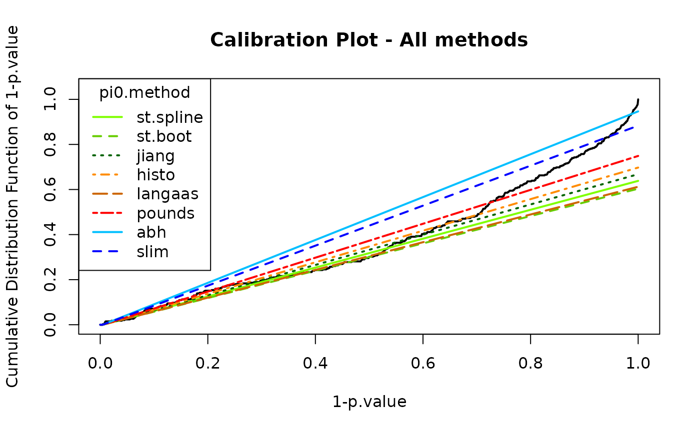
calibration_all$pi0## pi0.Storey.Spline pi0.Storey.Boot pi0.Jiang pi0.Histo pi0.Langaas pi0.Pounds
## 1 0.6383234 0.6035503 0.6679852 0.6973795 0.6122122 0.7489547
## pi0.ABH pi0.SLIM
## 1 0.9467456 0.8832706In some situations, the curve may not show a sufficiently sharp increase, or the entire distribution may be ill-calibrated. In some cases, the issue may stem from earlier preprocessing steps.
If the increase is not strong enough but remains acceptable, it is possible to compensate for poor calibration by overestimating π0.
In the worst case, the Benjamini–Hochberg option can always be selected. This correspond to the safer case of π0=1, which is not shown on the previous plot as it always corresponds to a diagonal line.
The histPValue_HC() function provides an alternative
graphical representation of the distribution of p-values and π0, while
conveying the same information. It is more intuitive to understand, but
more difficult to use it to precisely assess the calibration quality.
Both graphics are thus complementary.
 #chosen pi0
pi0 <- 1

 #calibration plot with chosen method
wrapperCalibrationPlot(vPVal = pval_nopush,
                       pi0Method  = pi0)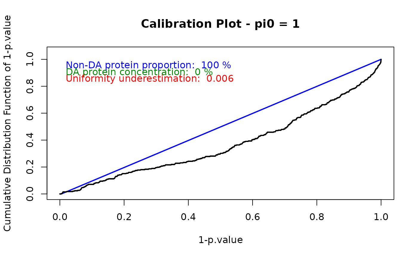
## $pi0
## [1] 1
##
## $h1.concentration
## [1] 0
##
## $unif.under
## [1] 0.006418716
 #histogram of p-values density
histPValue_HC(pval_nopush,
              bins = 50,
              pi0 = pi0
)
The diffAnaComputeAdjustedPValues() function returns the
adjusted p-values corresponding to the p-values of the differential
analysis. Proteins with a logFC below the previously defined threshold
are taken into account when calculating adjusted p-values. However,
their p-value is pushed to 1, as they are considered ‘discarded’.
 #push to 1 proteins with logFC under threshold
pval_pushfc <- pval
pval_logfc_inf_ind <- which(abs(res_pval_FC$logFC) < Foldchange_thlogFC)
pval_logfc_inf_ind <- setdiff(pval_logfc_inf_ind, pushedpval_ind)
pval_pushfc[pval_logfc_inf_ind] <- 1
 #remove pushed p-values
pval_pushfc <- pval_pushfc[-pushedpval_ind]


 #calculate adjusted p-values
adjusted_pvalues <- diffAnaComputeAdjustedPValues(
  pval_pushfc,
  pi0)
## Procedure of Benjamini-Hochberg is used. pi0 is fixed to 1.
adjusted_pvalues_comp <- unlist(res_pval_FC$P_Value)
adjusted_pvalues_comp[-pushedpval_ind] <- adjusted_pvalues
FDR control
The final step is FDR control, which aims to limit the proportion of false positives among proteins identified as differentially abundant.
A p-value threshold is first defined to select the proteins deemed differentially abundant. Any protein with a p-value below this threshold is retained. The associated FDR level is then provided, based on the p-value adjustment procedure.
The expected number of false discoveries can be estimated by multiplying the FDR with the number significant proteins. Because the FDR is a percentage-based measure, it becomes difficult to interpret when the expected number of falsely discovered proteins falls below 1, as it corresponds to strictly less than one expected false discovery. This is likely to happen in small datasets. However, an FDR that becomes meaningless does not invalidate the proteomics experiment itself. It only means that the FDR should be used cautiously.
 #define p-value threshold
pval_threshold <- 0.01
FDRcontrol_thpval <- -log10(pval_threshold)

 #get FDR
pval[pushedpval_ind] <- 1
logpval <- -log10(pval)
logpval_thpval_ind <- which(logpval >= FDRcontrol_thpval)
logpval_thpval_ind <- setdiff(logpval_thpval_ind, pval_logfc_inf_ind)
fdr <- diffAnaComputeFDR(adjusted_pvalues_comp[logpval_thpval_ind])

 #determine differentially abundant proteins
isDifferential <- is.differential(pvalue = pval,
                                 logFC = res_pval_FC$logFC,
                                 thpvalue = FDRcontrol_thpval,
                                 thlogFC = Foldchange_thlogFC)
NbSignificant <- length(which(isDifferential == 1))

cat("pvalue threshold : ", pval_threshold, "\n",
    "logpvalue threshold : ", FDRcontrol_thpval, "\n",
    "FDR : ", round(100*fdr, 2), "%\n",
    "Number significant proteins : ", NbSignificant, "\n",
    "Number of expected false discovery : ", fdr*NbSignificant, "\n")
## pvalue threshold : 0.01
## logpvalue threshold : 2
## FDR : 16.75 %
## Number significant proteins : 19
## Number of expected false discovery : 3.18342The diffAnaVolcanoplot_rCharts() function provides a
volcano plot to visualize the differentially abundant proteins according
to the logFC and p-value thresholds. It requires a
data.frame containing the logFC, log-transformed p-values,
protein index, and any additional information to be displayed in the
tooltip when hovering over a point in the plot. The FDR threshold
corresponds to the horizontal dashed line, and the logFC threshold to
the vertical dashed line.
 #create dataframe for volcano plot
df <- data.frame(
  x = unlist(res_pval_FC$logFC),
  y = logpval,
  index = as.character(rownames(obj[[length(obj)]]))
  )
tooltip <- "proteinId"
df <- cbind(df, SummarizedExperiment::rowData(obj[[length(obj)]])[, tooltip, drop = FALSE])
colnames(df) <- gsub(".", "_", colnames(df), fixed = TRUE)
if (ncol(df) > 3) {
  colnames(df)[4:ncol(df)] <- paste0("tooltip_",
                                      colnames(df)[4:ncol(df)])
}
cond <- unique(design.qf(obj)$Condition)

 #volcano plot
diffAnaVolcanoplot_rCharts(
  df,
  th_pval = FDRcontrol_thpval,
  th_logfc = Foldchange_thlogFC,
  conditions = cond
)
A new assay can be created to keep all values of interest, such as all p-values, logFCs, or the differential or non-differential status of each protein. This allows you to keep this data organized in a single object and reuse it later if necessary for further processing or visualization.
 #create new assay with all values of interest
obj <- QFeatures::addAssay(obj, obj[[length(obj)]], 'DifferentialAnalysis')
SummarizedExperiment::rowData(obj[[length(obj)]])$pval <- unlist(res_pval_FC$P_Value)
SummarizedExperiment::rowData(obj[[length(obj)]])$logpval <- logpval
SummarizedExperiment::rowData(obj[[length(obj)]])$logFC <- unlist(res_pval_FC$logFC)

SummarizedExperiment::rowData(obj[[length(obj)]])$adjusted_pval <- adjusted_pvalues_comp

SummarizedExperiment::rowData(obj[[length(obj)]])$isDifferential <- isDifferential

obj
## An instance of class QFeatures (type: bulk) with 8 sets:
##
## [1] original: SummarizedExperiment with 500 rows and 6 columns
## [2] logAssay: SummarizedExperiment with 500 rows and 6 columns
## [3] Filtered: SummarizedExperiment with 480 rows and 6 columns
## ...
## [6] aggregated: SummarizedExperiment with 378 rows and 6 columns
## [7] FilterProt: SummarizedExperiment with 357 rows and 6 columns
## [8] DifferentialAnalysis: SummarizedExperiment with 357 rows and 6 columnsSession information
## R version 4.5.2 (2025-10-31)
## Platform: x86_64-pc-linux-gnu
## Running under: Ubuntu 24.04.3 LTS
##
## Matrix products: default
## BLAS:   /usr/lib/x86_64-linux-gnu/openblas-pthread/libblas.so.3
## LAPACK: /usr/lib/x86_64-linux-gnu/openblas-pthread/libopenblasp-r0.3.26.so;  LAPACK version 3.12.0
##
## locale:
##  [1] LC_CTYPE=C.UTF-8       LC_NUMERIC=C           LC_TIME=C.UTF-8
##  [4] LC_COLLATE=C.UTF-8     LC_MONETARY=C.UTF-8    LC_MESSAGES=C.UTF-8
##  [7] LC_PAPER=C.UTF-8       LC_NAME=C              LC_ADDRESS=C
## [10] LC_TELEPHONE=C         LC_MEASUREMENT=C.UTF-8 LC_IDENTIFICATION=C
##
## time zone: UTC
## tzcode source: system (glibc)
##
## attached base packages:
## [1] stats     graphics  grDevices utils     datasets  methods   base
##
## other attached packages:
## [1] DaparToolshed_0.99.24 BiocStyle_2.38.0
##
## loaded via a namespace (and not attached):
##   [1] RColorBrewer_1.1-3          geeM_0.10.1
##   [3] jsonlite_2.0.0              MultiAssayExperiment_1.36.1
##   [5] magrittr_2.0.4              shinyjqui_0.4.1
##   [7] MESS_0.6.0                  farver_2.1.2
##   [9] rmarkdown_2.30              geepack_1.3.13
##  [11] fs_1.6.6                    ragg_1.5.0
##  [13] vctrs_0.7.1                 multtest_2.66.0
##  [15] forcats_1.0.1               htmltools_0.5.9
##  [17] S4Arrays_1.10.1             BiocBaseUtils_1.12.0
##  [19] progress_1.2.3              haven_2.5.5
##  [21] curl_7.0.0                  broom_1.0.12
##  [23] SparseArray_1.10.8          TTR_0.24.4
##  [25] sass_0.4.10                 bslib_0.10.0
##  [27] htmlwidgets_1.6.4           basilisk_1.22.0
##  [29] desc_1.4.3                  plyr_1.8.9
##  [31] zoo_1.8-15                  lubridate_1.9.5
##  [33] cachem_1.1.0                cp4p_0.3.6
##  [35] igraph_2.2.1                mime_0.13
##  [37] lifecycle_1.0.5             pkgconfig_2.0.3
##  [39] Matrix_1.7-4                R6_2.6.1
##  [41] fastmap_1.2.0               shiny_1.12.1
##  [43] MatrixGenerics_1.22.0       clue_0.3-66
##  [45] digest_0.6.39               S4Vectors_0.48.0
##  [47] textshaping_1.0.4           GenomicRanges_1.62.1
##  [49] invgamma_1.2                filelock_1.0.3
##  [51] Spectra_1.20.1              timechange_0.4.0
##  [53] abind_1.4-8                 compiler_4.5.2
##  [55] withr_3.0.2                 fontquiver_0.2.1
##  [57] S7_0.2.1                    backports_1.5.0
##  [59] BiocParallel_1.44.0         MASS_7.3-65
##  [61] DelayedArray_0.36.0         tools_4.5.2
##  [63] PSMatch_1.14.0              otel_0.2.0
##  [65] httpuv_1.6.16               zip_2.3.3
##  [67] quantmod_0.4.28             clipr_0.8.0
##  [69] glue_1.8.0                  promises_1.5.0
##  [71] QFeatures_1.20.0            grid_4.5.2
##  [73] ggformula_1.0.1             cluster_2.1.8.1
##  [75] reshape2_1.4.5              generics_0.1.4
##  [77] gtable_0.3.6                labelled_2.16.0
##  [79] preprocessCore_1.72.0       tidyr_1.3.2
##  [81] data.table_1.18.2.1         hms_1.1.4
##  [83] MetaboCoreUtils_1.18.1      XVector_0.50.0
##  [85] BiocGenerics_0.56.0         pillar_1.11.1
##  [87] stringr_1.6.0               limma_3.66.0
##  [89] later_1.4.5                 splines_4.5.2
##  [91] dplyr_1.2.0                 lattice_0.22-7
##  [93] survival_3.8-3              tidyselect_1.2.1
##  [95] fontLiberation_0.1.0        knitr_1.51
##  [97] fontBitstreamVera_0.1.1     bookdown_0.46
##  [99] IRanges_2.44.0              Seqinfo_1.0.0
## [101] ProtGenerics_1.42.0         SummarizedExperiment_1.40.0
## [103] stats4_4.5.2                xfun_0.56
## [105] Biobase_2.70.0              statmod_1.5.1
## [107] mosaicCore_0.9.5            matrixStats_1.5.0
## [109] stringi_1.8.7               Pirat_1.4.4
## [111] lazyeval_0.2.2              yaml_2.3.12
## [113] evaluate_1.0.5              codetools_0.2-20
## [115] qvalue_2.42.0               MsCoreUtils_1.22.1
## [117] gdtools_0.4.4               tibble_3.3.1
## [119] BiocManager_1.30.27         graph_1.88.1
## [121] cli_3.6.5                   xtable_1.8-4
## [123] reticulate_1.44.1           systemfonts_1.3.1
## [125] jquerylib_0.1.4             Rcpp_1.1.1
## [127] dir.expiry_1.18.0           png_0.1-8
## [129] parallel_4.5.2              pkgdown_2.2.0
## [131] ggplot2_4.0.2               assertthat_0.2.1
## [133] prettyunits_1.2.0           AnnotationFilter_1.34.0
## [135] ggiraph_0.9.4               rlist_0.4.6.2
## [137] scales_1.4.0                xts_0.14.1
## [139] ggridges_0.5.7              openxlsx_4.2.8.1
## [141] purrr_1.2.1                 highcharter_0.9.4
## [143] crayon_1.5.3                rlang_1.1.7